3 Storage And Retrieval

A simple Append-Only log db

Each (key, value) inserts are appended in a static file
While searching, the last value corresponding to key is returned
O(1) insertion but fails terribly in search and deletion with O(n).
Too much memory consumption too.

Hash Indexes

Indexes solves the problem of searching through the db for a key.
Uses hash table to map key to byte offset of corresponding key's value.
```
                  key --> byte offset of value 
```

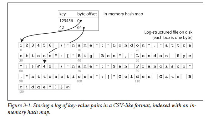
On insertion, hash map is updated with the new offset and lookup can be done in O(1).
Engines like Bitcask uses this approach.
Useful when there aren't many keys but each key has many writes
To solve the memory consumption problem, we break down the db into multiple files after each file reaches a certain limit.
Better approach is to use Compaction where we store only the latest value of a key by taking all the segments and merging their values (something like MapReduce).

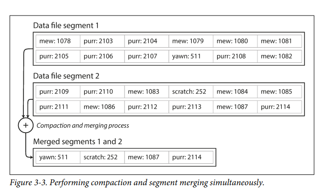
For supporting deletion, a seperate record called tombstone is maintained which specifies merge operations to skip the values which are already deleted.
For supporting concurrency, only one write thread is maintained and reading can be done concurrently.

Advantages of Append-Only design

Even though this design seems bad, appending and segment merging seems to be faster than performing random writes in a ssd.
Concurrency and crash recovery are simpler.

Limitations of Append-Only design

Might run out of memory in hash table if we have large number of keys.
Range queries are not efficient. Ex: find all keys between A1 - A100.

SSTables and LSM-Trees

Sorted String Tables

keys are sorted in ascending order instead of using hash indexes
In the compaction process, first key of each file is compared simultaneously and then the lowest one is put into the merged file. This ensures we take the most recent values of keys as well as keys are in sorted order.

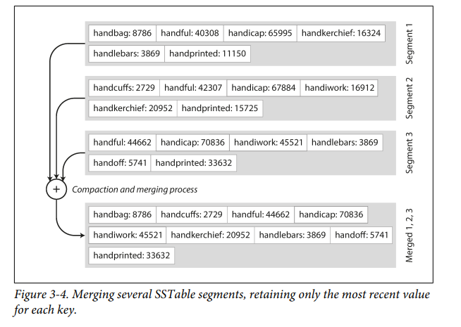
Searching keys is easier as all keys are sorted and we needn't store all hash indexes in memory.

Constructing and maintaining SSTables

Its kinda simple yet beautiful. To maintain the sorted keys we use AVL or red-black trees in memory (!! not in disk). Called as memtable.
When the size grows bigger, we write the memtable onto the disk as a new segment file as a background process.
Log is also maintained to recover the not-written in-memory data when system crashes.
For searching, we first check the memtable, then most recent segment, and second-most recent segment and so-on.
To improve search, we can do the compaction process from time to time.

Making an LSM-tree out of SSTables

LSM - ==Log Structured Merge-Tree==
Basically the name for practical implementation of SSTables
For keys non existent in the db, search all the way back to oldest segment is needed. To avoid that, bloom filters are used which tells whether a key is present or not approximately.

B-Trees

Stores key-value pairs sorted by keys similar to SSTables.
B-Trees break the database into fixed-size blocks or pages.
Each page is mostly 4KB in size.
Reads or writes one page at a time.
Each page has an address identifier which allows one page to refer to another. It is stored on disk not memory.
We can use these page refs to construct a tree.

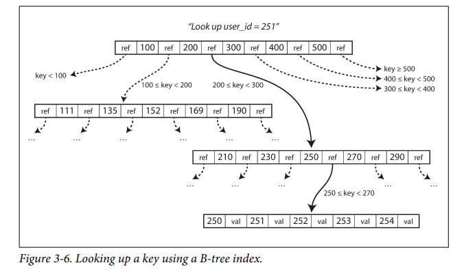
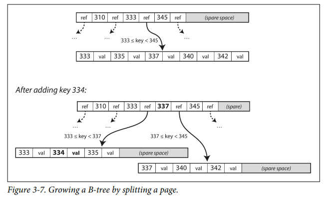
The number of references to child pages in one page of the B-tree is called the branching factor.
If inserting a new record exceeds the space limit of 4KB, then the page is split into 2 halves.

Making B-trees reliable

Write operation - overwrite a page on disk with new data
Some write operations like insert needs many pages to be updated (cases where a page is split into 2 halves).
This is vulnerable to crashes and there will be corrupted index after crashes
To prevent that, B-Trees use WAL (Write-Ahead log). This is an append-only log file where every B-Tree modification is stored before actually performing it. It is used to recover data after crashes.

Comparing B-Trees and LSM-Trees

Generally, LSMs are faster for writes and B-Trees are for reads.

Advantages of LSM-Trees

B-Tree index has more write overhead due to 2 writes , one to the b-tree itself and another one to the WAL.
LSM-Trees also have to rewrite data multiple times during compaction and merging phase.
This effect—one write to the database resulting in multiple writes to the disk over the course of the database’s lifetime — is known as write amplification.
LSM-Trees have less write amplification because it is sequential and sequential writes are faster than random writes.
LSM-Trees can be compressed and result in smaller files but B-trees leave some storage unused in each page (due to fragmentatin).

Disadvantages of LSM-Trees

Compaction process can affect reads and writes while its taking place as it is an expensive process and takes most of the disk's bandwidth.
B-Trees has only one copy of each key whereas LSM has many copies of a key.

Other Indexing Structures

Secondary Index

Keys other than primary keys can be indexed - Secondary indexes.
Each index can either contain a row (or document, vertex) or it could contain a reference which points to it
Generally the rows itself are stored somewhere else called heap file and the indexes have reference to the rows.
Avoids duplicate data and inconsistency.
Issue comes when an update (updating data) happens but it exceeds the space limit in that segment, then the data is moved to a new location where there is enough space and either all pointers are updated or a forwarding pointer is stored in place of old value which points to address of new pointer.
This extra hop (mentioned in previous example) is expensive. So, its desirable to have indexed row directly within an index. Knows as clustered index.
MySQL InnoDB always stores the primary key as clustered index and all secondary indexes point to the primary key and not heap file.

Multi-Column Index

Needed when multiple column conditions are specified in the query.
Concatenated Index - some columns are concatenated into a single value and stored as index. This will work only for any starting prefix of columns (in which they are stored in index) and not any particular order. Ex: if we concatenate indexes for (first_name,last_name) we can either query for first_name or first_name + last_name but not last_name because of the ordering of column in the index.

For the above query, Traditional B-Trees indexing are inefficient cuz they can either query for latitude or longitude but not both as they index only one key.

Full-text search and fuzzy indexes

All indexes and search till now are for exact match with keys
Fuzzy Search - Match similar keys
Full Text Search - search for one word could be to include synonyms, ignore grammatical variations of the words.

Memory Databases

Disks - durable, cost efficient but very awkward to deal with.
If size of db is less, they can be stored in memory distributed over serveral machines - memory databases.
Memcached : In-memory key-value store used for caching.
Memory dbs can be extended to have more size than RAM also by evicting the LRU data onto disk thus cleaning up more memory.

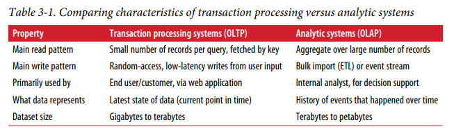
Transaction Processing or Analytics?

OLTP - Online transaction processing
OLAP - Online Analytics processing

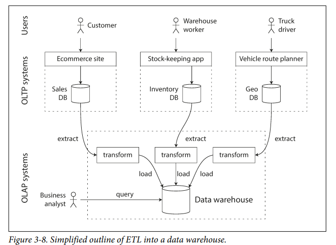
Data Warehousing

A large company may contain so many OLTP dbs. For analytics purpose, data from those dbs are extraced periodically and stored in a warehouse db specifically made for analytics.

Divergence between OLTP databases and data warehouses

Data model for data warehouse is mostly relational
SQL - good fit
Engines - Teradata, Vertica, SAP HANA, and ParAccel

Stars and Snowflakes: Schemas for Analytics

==Star Schema== : Schema structure like Star, Fact-Table in middle and dimensional-tables surrounding that. Most commonly used.
==Snowflake Schema== : dimensions are broken down into sub-dimensions.

Column-Oriented Storage

Most OLTP dbs are stored in row-oriented fashion.
OLAP mostly needs 4-5 columns out of 100s of columns in each row and they also aggregate all the column values together. So its more efficient to use column-oriented storage technique here.

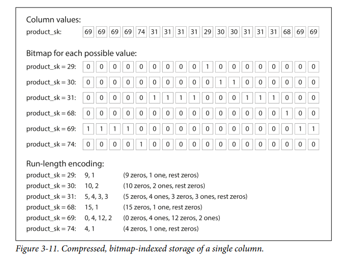
Column Compression

Bitmap encoding can be used to compress the column values further

Memory bandwidth and vectorized processing

Column oriented storage helps in making good efficient use of CPU cycles.

Sort Order in Column Storage

Sorting according to a specific column helps in doing range queries.
Data needs to be sorted entire row at a time in column oriented storage as each column's positioning has to be consistent with each other.

Writing to Column-Oriented Storage

Though reads for analytics purpose are efficient in column-oriented storage, writes are very inefficient.
For each row to be updated / inserted, we need to update all columns.
Using a LSM-Tree based approach will be better for writes as all data first goes into an in-memory store, where they are added to sorted structure.

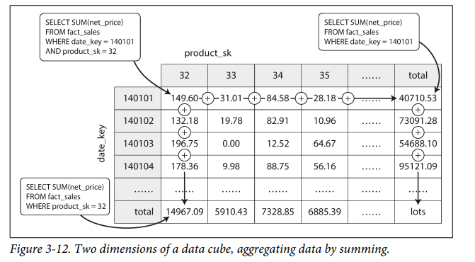
Aggregation: Data Cubes and Materialized Views

Warehouses mostly queries aggregate values of data.
It's sometimes efficient to cache the aggregated values beforehand.